This assignment had multiple tasks to teach the student many aspects of working with different remotely sensed images. The first task taught the student how to decipher their selected study area out of a a large satellite aerial image. The second taught how to optimize the resolution images. With a higher resolution, it allows for easier visual interpretation. Radiometric enhancement was the third technique that was taught in the assignment. The students were taught how to link Google Earth with Erdas Imagine for more aerial interpretation. Multiple methods of image mosaicking were taught to the students. The final task for this assignment was working with binary change. This change was then mapped using ArcMap.
Methods:
The first method that was used was image subsetting or creating an areas of interest within a particular study area. For this particular example Chippewa and Eau Claire County were chosen as the area of interest. The image below (Figure 1) shows the results of this process.
 |
| Figure 1. Shows the results of subsetting an area within a study area. |
The second step involved increasing the spatial resolution of an image. The first image used had a 30 meter resolution while the second image had a 15 meter resolution. By resampling the images it allowed for the original image to have a more crisp appearance. With a higher spatial resolution, it allows for easier aerial photo interpretation.
The third step was a basic radiometric enhancement of a particular image. The technique used was haze reduction. After running this tool, it allowed for the image to appear clearer and more crisp. It did not have a higher spatial resolution, but by reducing the haze it gave it the appearance of having a higher resolution.
The next step involved linking Google Earth with the Erdas Imagine image viewer. Once the views were linked, it allowed for a different form of aerial interpretation to take place.
The sixth task was image mosaicking. Two images were provided from May 1995. The two different techniques there were used were mosaic express and mosaic pro. The image below (Figure 2) shows the results of the mosaic express.
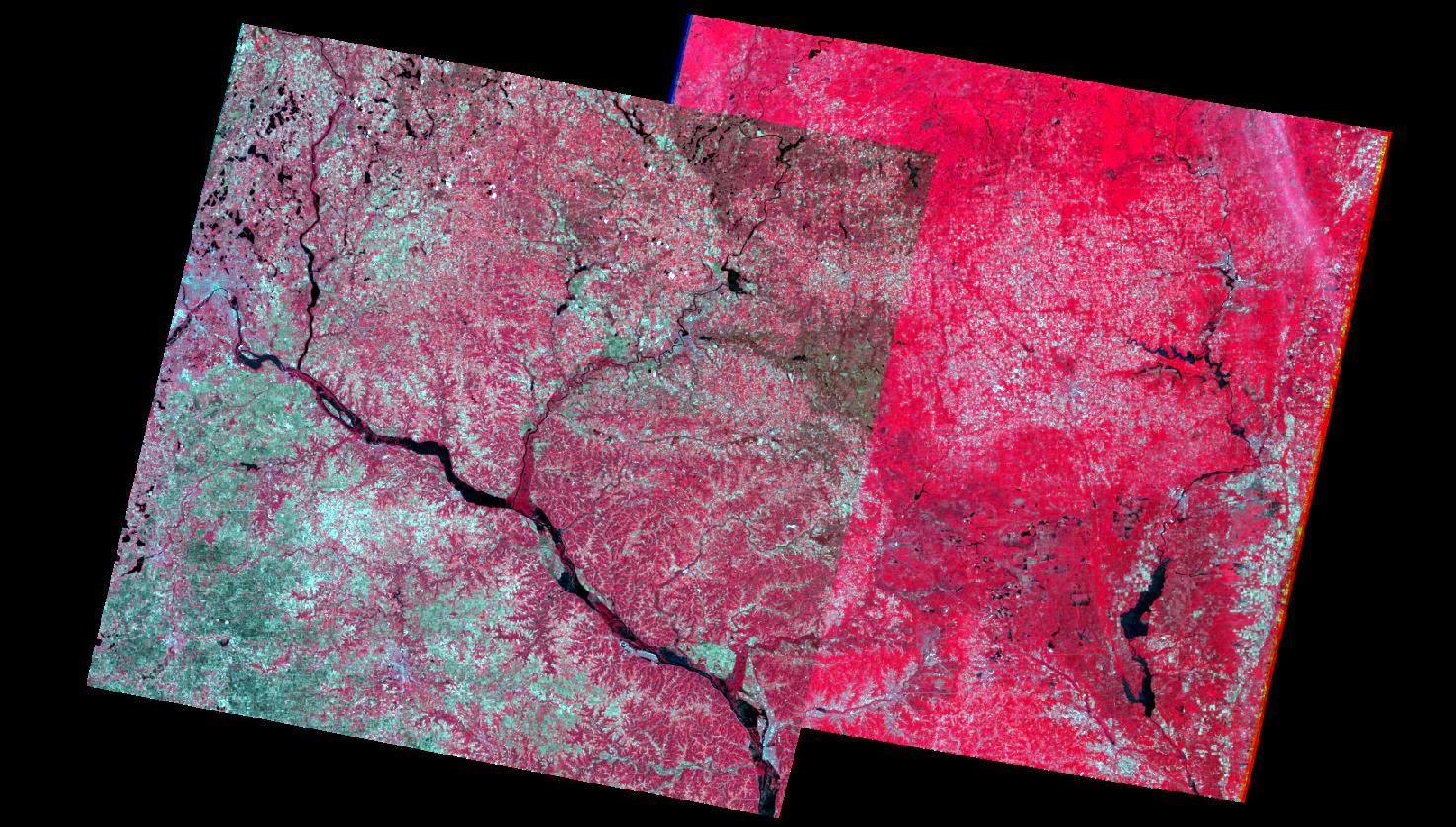 |
| Figure 2. This image is the result of mosaic express. There is not a gradual combining of the images and a very distinct boundary between the two. |
The results of this process were not mixed together very well. The two images have two different color schemes and do not blend well together. The figure below (Figure 3) shows the results of using mosaic pro.
 |
| Figure 3. This is the result of mosaic pro. The images are blended together much smoother and the color scheme is much similar between the two images. |
These two images blend together much better than figure 2. The color schemes are very similar and there is not as distinct of a line between the two different images. There were many more options to choose how the blended together using mosaic pro.
The final step in the assignment involved image differencing or binary change detection. The particular are being analyzed included Eau Claire County and four other neighboring counties. The difference will be conducted between the years of 1991-2011. In order to see where these changes fall, it is necessary to look at the metadata. The graph below (Figure 4) is a histogram of the data for the image differencing.
 |
| Figure 4. This is a histogram of the metadata showing where the tails are located that dictate whether there was change or not on the land. |
The differences typically fall on the tails of the graph. The tails are marked by vertical red lines. Values greater than 75.049 and lower than 27.789 are considered to be changed areas.
Although the histogram shows what values represent change, it is not easy to see without mapping this particular data. The map below (Figure 5) shows the results of the image differencing. Many of the changes that occurred happened in rural areas of the selected counties.
 |
| Figure 5. This is the map showing which areas experienced change and which areas did not. |
Sources: Earth Resources Observation and Science Center, United States Geological Survey
Mastering ArcGIS 6th edition Dataset by Maribeth Price, McGraw Hill. 2014.
No comments:
Post a Comment